Often, when studying people’s subjective experiences, data are collected by asking survey participants to report on an ordinal scale how much they agree with a statement or question. For example, you might ask a question like this:
On a scale of 1 to 10, how hungry are you right now?
Not at all hungry Very hungry
1 2 3 4 5 6 7 8 9 10
In this post I’ll use the example of comparing self-reported happiness between countries. These data were collected by the World Values Survey (Inglehart et al., 2014), using the following question:
Taking all things together, would you say you are
1 Not at all happy
2 Not very happy
3 Rather happy
4 Very happy
Applications of this are abundant in business (Net Promoter Score), social science (Likert scales, survey data), and even medicine (pain scales). Now, one interesting question with this kind of data is, given two sets of responses, how do you determine which one is greater than the other on average?
That might sound easy, but it’s hard. Because the data are on an ordinal scale, all we know is that each successive value is greater than the previous one, but not by how much. Therefore, the mean response is not well defined. You could use the median, but often the medians of two groups will fall within the same category even though there really is a difference. In the literature on self-reported happiness, many researchers have resorted to hacky solutions like taking the simple mean (Leigh and Wolfers, 2006; Inglehart et al., 2008), applying an arbitrary cutoff to make the data binary (Inglehart & Klingemann, 2000; Yang, 2008) or simply applying linear regression to the numerical encoding of the responses (Napier and Jost, 2008). These methods either throw out a lot of data or else wrongly treat the ordinal data as if they were interval data.
A more sophisticated approach is to assume that, underlying people’s discrete responses, there is some continuous latent variable, which we’ll denote y. We can further assume that y is normally distributed in each group (for a single group, you can arbitrarily scale y to enforce this condition; the requirement that y be normally distributed in all groups is a further assumption of the model), and that there exist thresholds t1, t2, … tM-1 such that someone with y < t1 reports the lowest level, someone with t1 < y < t2 reports the second level, and so on. Then, we can use ordered probit regression to jointly estimate the group means of y, the variance of y, and thresholds that best explain the observed data. Once the model is fit, we can then compare the estimated means of y for each group.
However, as Bond and Lang (2014) point out in their scathing paper, “The Sad Truth about Happiness Scales,” there is still a serious problem. Usually, two (or more) groups will differ not only in mean, but also in variance. This condition (called heteroskedasticity) implies that any claims about differences in mean happiness will depend on the arbitrary choice of normal distribution for the latent variable, and they will be reversible under other, equally valid choices. Why is that? It’s always possible to choose a different cardinalization that stretches the scale while preserving the rank order (for example, you can transform the normal distribution to a skewed distribution such as the log-normal). Bond and Lang prove that when the variances are unequal, you can easily choose transformations under which either distribution comes out with a higher mean. Moreover, all of these transformations are equally valid because the data are on an ordinal scale, which doesn’t distinguish among monotonic transformations.
Let’s visualize this idea. First consider two normal distributions: the red distribution has mean 0 and variance 15, and the blue distribution has mean 10 and variance 30.

Next we apply a log-normal transformation that skews the distribution to the right. This exaggerates the mean difference between the blue and red curves:

We can also apply the corresponding transformation skewing the distribution to the left, and now the mean of the blue distribution is actually lower! Because each of the three plots is equally consistent with an ordinal dataset, we can’t meaningfully claim that either of the two curves “really” has a higher mean.

Finally, Bond and Lang show that many existing findings in the happiness literature can be reversed, or at least made not statistically significant, by introducing plausible amounts of skewness (i.e. no more skewed than the income distribution) to the latent variable. In particular, using the World Values Survey 2005 data, they show that the ranking of countries by mean happiness is unstable to variations in the skewness parameter.
In summary: Although we have a statistical method (ordered probit regression with heteroskedasticity) for modeling ordinal response scales, it doesn’t say anything about the differences between groups on average. In the next section, I’ll use the happiness example to explore what we can say about the data.
Methods and Results
The data consist of subjective happiness reports for 83097 participants on a scale of 1 to 4, from 58 countries. The model was fit using the oglmx package in R (Carroll, 2018). The model implements ordered probit regression with heteroskedasticity. This estimates the mean and standard deviation of the latent variable for each country (no other covariates were included). Of the three thresholds between the four response levels, the first is also estimated by the model, while the other two are normalized to 1 and 2. R code implementing the analyses in this post, as well as some validation of the methods on simulated data, is available here.
As a first descriptive result, how does our model fit relate to simpler happiness statistics? The following table shows correlations between the model parameters and other summary metrics of national happiness:

A few things stand out. First, all four summary statistics are positively correlated at least at r = .55. Second, mean latent happiness is almost perfectly correlated (r = .98) with the simple mean of the responses. That suggests it’s probably not worth the trouble to fit the model just to use mean latent happiness as a summary statistic. Finally, the standard deviation of latent happiness is correlated – in different directions – with all four summary statistics. That means no summary statistic can be taken at face value and assumed to be unbiased by variance!
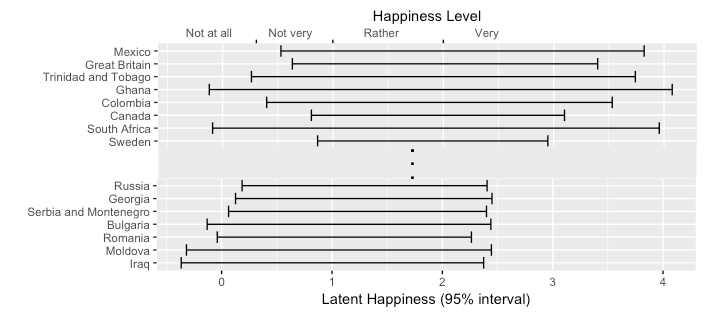
Next, we can plot, for each country, the interval containing 95% of the latent happiness values:

We can see that countries vary quite a bit in both mean and spread. The plot is shown sorted by mean, but sorting by the interval endpoints (i.e., 2.5 and 97.5 percentile) give different rankings: high-variance countries (Ethiopia, Turkey, Mali, South Africa, Ghana, Mexico, Trinidad and Tobago) would rank much lower if sorted by the lower bound, and higher if sorted by the upper bound. This instability is similar to Bond and Lang’s analysis of instability under different degrees of skewness. However, the instability isn’t random: it’s directly related to the variance of each country. That suggests it might be useful to think of the result as a pair (mean, variance), rather than trying to estimate the mean in spite of the variance. Then it makes sense to plot mean latent happiness against its standard deviation in a scatterplot:

There are some obvious patterns here. Countries in Latin America and Africa tend to have the highest standard deviations, whereas East and Southeast Asian countries have low standard deviations. That might be either because of actual differences in happiness inequality, or cultural differences in tendency to report extreme values. Eastern European countries tend to have low mean happiness. Rich, stable, egalitarian developed countries (Norway, New Zealand, Sweden, Canada) tend to have high means and low standard deviations, indicating that most people there report being at least content, if not extremely happy.
Next, can we answer our original question of ranking two groups? The problem with the mean y is, fundamentally, that it’s an “interval” answer to an ordinal problem: it is sensitive to the distribution of y, yet this distribution is chosen arbitrarily because the data specify only rank. A more “non-parametric” answer is to instead compute the probability that a random person from country A is happier than a random person from country B. Let’s call that the “win probability” (WP is also known as the common language effect size, because apparently the statistician who invented thought it was that intuitive). We can say that people from country A report being happier than people from country B if WP of A over B is greater than 0.5. Moreover, this conclusion will not be changed by monotonic transformations of the latent variable. Win probability between two independent normal distributions can be computed as follows:
Let
a ~ N(μa,σ2a)
b ~ N(μb,σ2b)
If a and b are independent then
a – b ~ N(μa – μb, σ2a + σ2b)
and
WP = P(a – b > 0).
Thus finding WP is equivalent to computing the CDF of the normal distribution.
We can also estimate a confidence interval for WP by Monte Carlo simulation: the ordered probit regression outputs the covariance matrix of the model coefficients, from which we can sample coefficient values according to a multivariate Gaussian. We compute WP for each sample, and then construct an interval that contains the middle 95% of all samples.
This allows us to answer our original question of whether one country is “happier” than another. You could say that a country is happier when win probability is greater than 0.5, but this gives counterintuitive results when the variances are different, and requires you to care only about the rank order and not the magnitude of differences. A stronger condition is to say that country A is happier than country B when win probability is significantly greater than 0.5 and the 2.5th and 97.5th percentiles of the latent variable distribution are both greater for country A than B.
We can plot the win probability of all other countries against a fixed comparison country, and color-code by our condition for declaring group differences:

Conclusion
The above results are consistent with other surveys of self-report happiness, suggesting that the underlying survey results are robust, whereas the interpretation hides the greatest difficulty. The most prominent example is probably the UN World Happiness Report and its associated Happiness Index (Helliwell et al., 2018). This is calculated using the simple mean of an ordinal scale ranging from 1 to 10. Although the Index is usually used directly as a measure of overall happiness, we can see that their data demonstrate the same patterns of variable spread. The following plot comes from the UN’s population-weighted regional estimates of happiness:

Again, North American countries have a higher mean response, whereas Latin American and Caribbean countries have a higher standard deviation. As we’ve seen, that means we can confidently say (for example) that Canadians report being happier than Americans, whereas any index claiming to determine which of Americans and Mexicans report being happier is highly suspect at best.
Ordered probit regression is a powerful method for analyzing ordinal-scale subjective data, but the results must be interpreted with care. It is not generally valid to summarize the results using the model’s estimated mean for each group, and claim that higher estimated means indicate more of the response’s underlying driver. Instead, the mean and variance must be interpreted jointly according to the application. The visualizations in this post are an example of this interpretation for the test case of national happiness survey data. I introduce a rule of thumb for claiming that a true difference exists between groups. Of course, in this context I mean a difference between countries in reported happiness, which may be caused either by a difference in actual happiness or in the reporting function. Although the analyses in the post deal with responses as a function of only one categorical variable, the method can be used with multiple regression and both continuous and discrete predictors. Overall, one lesson from all this is that sometimes you have to make yourself ask the questions your data naturally answer, rather than make your data answer the questions you want to ask.
References
Bond, T. N., & Lang, K. (2014). The sad truth about happiness scales (No. w19950). National Bureau of Economic Research.
Carroll, N. oglmx (2018): A Package for Estimation of Ordered Generalized Linear Models.
Leigh, A., & Wolfers, J. (2006). Happiness and the human development index: Australia is not a paradox. Australian Economic Review, 39(2), 176-184.
Helliwell, J., Layard, R., & Sachs, J. (2018). World Happiness Report 2018, New York: Sustainable Development Solutions Network.
Inglehart, R., Foa, R., Peterson, C., & Welzel, C. (2008). Development, freedom, and rising happiness: A global perspective (1981–2007). Perspectives on psychological science, 3(4), 264-285.
Inglehart, R., C. Haerpfer, A. Moreno, C. Welzel, K. Kizilova, J. Diez-Medrano, M. Lagos, P. Norris, E. Ponarin & B. Puranen et al. (eds.). 2014. World Values Survey: All Rounds – Country-Pooled Datafile Version: http://www.worldvaluessurvey.org/WVSDocumentationWVL.jsp. Madrid: JD Systems Institute.
Inglehart, R., & Klingemann, H. D. (2000). Genes, culture, democracy, and happiness. Culture and subjective well-being, 165-183.
Napier, J. L., & Jost, J. T. (2008). Why are conservatives happier than liberals?. Psychological Science, 19(6), 565-572.
Yang, Y. (2008). Social inequalities in happiness in the United States, 1972 to 2004: An age-period-cohort analysis. American sociological review, 73(2), 204-226.