The way we use words in language encodes a lot of information about the real-world meaning of those words. After all, how else could we learn about things we’ve never experienced , just by reading or hearing about them? Although it’s controversial whether you can really know anything just by manipulating linguistic symbols without grounding them in experience, by finding structure in language we can generalize beyond our local environment.
One test case that researchers have used to illustrate this idea is the problem of estimating the locations of cities using distributional semantic vector embeddings of their names (Zwaan & Louwerse, 2005; Louwerse, Hutchinson, & Cai, 2012; Recchia & Louwerse, 2014). The Louwerse group’s general methodology for relating linguistic structure to geographic structure is as follows:
First, they create vector representations of city names using Latent Semantic Analysis (LSA). Then, they compute the cosine distances between each pair of cities. These are transformed using multidimensional scaling (MDS) so that they lie in a plane. Finally, they use bidimensional regression to compare the locations of cities in the linguistic plane to their actual locations. Bidimensional regression works by computing a transformation between the two spaces that maximizes the “correlation” between the two sets of city locations. To show that the result is statistically significant, they use a permutation test to find the distribution of optimal correlations when the two spaces are randomly shuffled with respect to each other (i.e. under the null hypothesis).
This method has a couple of drawbacks. First, the vector embeddings of city names are high-dimensional and do not lie on a plane, so reducing them using MDS throws away some of the structure encoded in the pairwise distances. Second, their statistical procedure only gives a p-value for the hypothesis that the correlation is greater than chance, but not a standard error or confidence interval for the estimate of the correlation strength.
In this post, I’ll propose a different method for characterizing how well distributional semantic vector representations of city names encode their geographic relations.
Methods
For the city locations, I downloaded the 100 most populous U.S. cities from Wikipedia. For the distributional semantics, I used Google’s pre-trained 1000-dimensional Word2Vec representations for real-world entities. The vectors are trained on a corpus of news articles. The Word2Vec representations are a little bit different from LSA in that they are based on words’ co-occurrences with other words rather than their distribution of occurrence across documents, but these differences won’t affect the analyses in this post.
One natural way to frame the problem is to ask: “Given two cities, if I know how distant they are in semantic space, can I predict how distant they are in geographic space?” Stated this way, we could proceed by computing the N x N matrix of pairwise cosine distances among semantic vectors, and the N x N matrix of pairwise geographic distances among N cities. Then, we can take the entries above the diagonal (below-diagonal entries are redundant because distance is symmetric) and flatten them into vectors of length 1/2(N2 – N). Then, the correlation between the semantic and geographic vectors is a measure of the correspondence between the two spaces. Additionally, we can compute regression coefficients and use the semantic distance to predict an estimate for the geographic distance.
You might object that this regression is invalid because the data points are not independent (e.g. on a plane, if we know the distance from a point X to three known points A, B, C, then we can determine the location of X). However, the regression coefficients still approximate what you would get if you could measure an infinite number of independent city pairs (ignoring the issue that there is in fact no infinite population of other American cities to draw from). Only the standard errors and p-values are wrong. We can use a Mantel test, based on random permutations, to test whether our estimated correlation is significantly greater than zero, and we can use bootstrap sampling to get a confidence interval around the estimate.
R code to perform the analyses in this post can be found here.
Results
First, a map of the 100 cities (omitting Anchorage and Honolulu:

Before computing the correlation between semantic and geographic distances, we should look at a scatterplot to check if the relationship is roughly linear and free of outliers:

Oops, there’s an obvious curvilinear relationship. Let’s try a log transform on the geographic distance:

That looks a little more reasonable. Linear regression of log(geographic distance) on normalized semantic distance gives:
log(dgeog) = 7.305 + 0.535 * dsem
The second coefficient means that for every additional standard deviation of semantic distance, the geographic distance should increase by a factor of e.535 = 1.708. We can also report the correlation coefficient of 0.61.
Is this effect significant? We can test it using a Mantel test. This test measures whether two pairwise distance matrices are correlated with each other. It works by randomly permuting the rows and columns of one matrix, which preserves its internal structure while wiping out any systematic relation to the other matrix. We repeat this many times, and then compare the actual value of the regression coefficient to the distribution of values it takes under permutations to get the p-value. I ran 1000 permutations, and the coefficient was far lower than the actual one 100% of the time, so the geographic structure encoded in language is statistically significant at least at p < .001.
We can also do better than that and generate a confidence interval around our estimate using bootstrap resampling. To do this, we randomly sample, with replacement, a set of 100 cities. The pairwise distances among these 100 cities (some of them duplicates) can be thought of as an approximation of the pairwise distances we would have gotten if we had picked a sample of 100 different cities from the original population (again ignoring the fact that those cities don’t exist). Then we compute the regression over the resampled distances (making sure to ignore cases where a city was compared to itself, as these distances are artificially zero). We repeat this many times, and the resulting distribution of regression coefficients approximates what we would have gotten if we could redraw from the population. Then the interval including the middle 95% of resampled regression coefficients approximates a 95% confidence interval for our measurement. This procedure gives a 95% confidence interval of (.450, .626), which means that for every additional standard deviation of semantic distance, the geographic distance should increase by a factor of 1.57 to 1.87.
This is a slightly unorthodox use of the bootstrap because the data are in a 2-dimensional matrix, so I also tested it on some simulated data (described in the Appendix) to confirm that it performs reasonably. This is a good thing to sanity check whenever you’re implementing a statistic that should have some specific distribution.
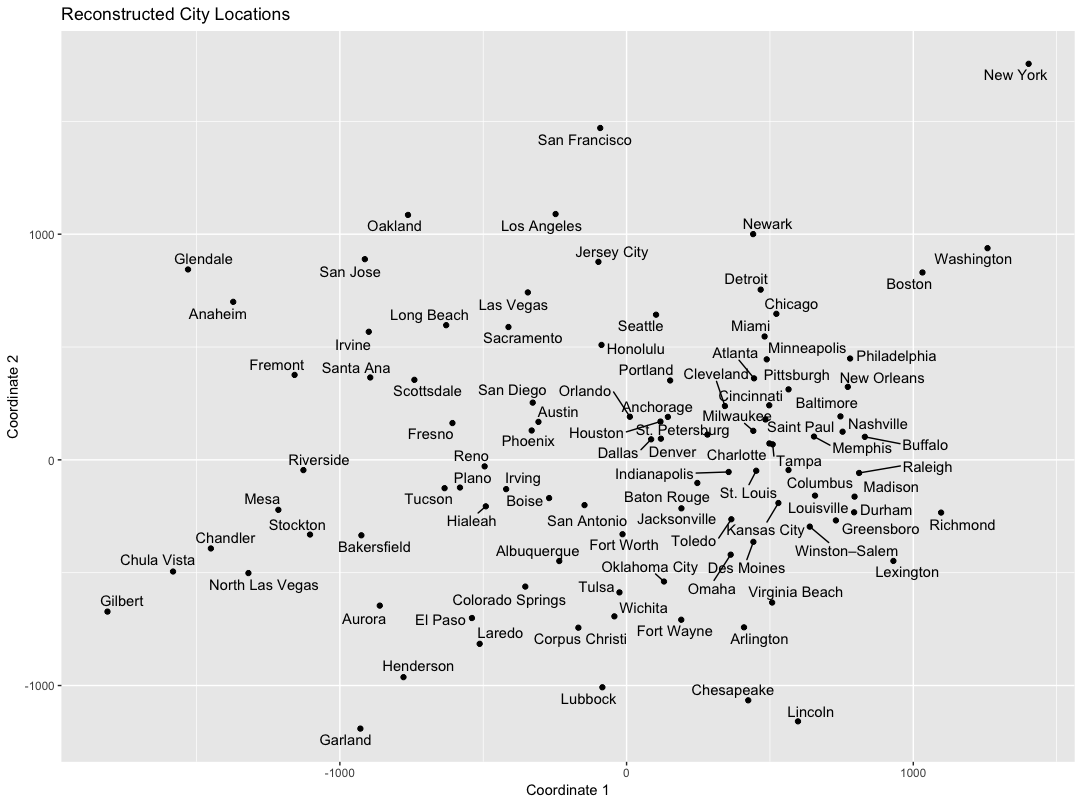
For fun, we can use our regression model to predict the distance between each pair of cities, and then use MDS to visualize a 2-dimensional approximation to the resulting “map” :

It’s far from perfect, but you can definitely see the Northeast, West Coast, West, and South/Midwest cities clustering together. Interestingly, the big cities of the West coast (San Jose, Oakland, Los Angeles, San Francisco, Seattle) appear closer to the Northeast (Newark, New York, Boston, Washington), suggesting that the semantic representations might be capturing similarities between the coastal population centers despite the long distance between them.
Conclusion
In this post, I demonstrated a method to determine how well semantic structure in texts encodes the geographic relations among U.S. cities. I replicated the main finding of Louwerse and Zwaan (2005), but with a different statistical framing of the problem, and introduced a confidence interval for the estimate of the effect. More generally, semantic similarity among words can encode information about other features of cities (Gupta, Boleda, Baroni, & Padó, 2015) or about other types of entities, such as social networks (Hutchinson, Datla, & Louwerse, 2012). The methods described in this post might also be used to compare the correspondence between any two pairwise relations. For example, you could predict:
• similarity between two people’s movie preferences given their similarity in demographic characteristics
• correlation between two neurons’ activity patterns given their similarity in gene expression
• correlation between two stocks’ price moves given their similarity in operating characteristics
The stats are more useful as a descriptive tool rather than for actual prediction, because you’d usually want to use the actual values of the known data points to predict the location of a new one, rather than relying on the pairwise distances.
Appendix: Checking bootstrapping performance on simulated data
I’ve claimed that the bootstrap confidence interval should contain the true value of the regression coefficient about 95% of the time. Rather than take this on faith in the math, we can do a simulation to make sure it works on a toy problem where the distribution is known. For this, I generated random data (x1, x2, x3, x4) according to a multivariate normal distribution with mean 0 and covariance matrix I + 3J, where J is a matrix of all ones. Now suppose we generate pairs, (x1, x2, x3, x4) and (x1’, x2’, x3’, x4’). We want to estimate the correlation between the two distances:
d1 = sqrt((x1 – x1’)2 + (x2– x2’)2)
d2 = sqrt((x3 – x3’)2 + (x4– x4’)2)
We can approximate the true value of this correlation ⍴ to arbitrary precision by generating many of these pairs. With the covariance matrix chosen, ⍴ = 0.67.
Next, I simulated the scenario in the post 1000 times. In each simulation, I generated 100 points, and computed the pairwise matrices of d1 and d2. The correlation r between the values of these matrices proved to be a good estimator of ⍴ (average r over 1000 simulations was 0.66). The bootstrap confidence interval for the correlation between d1 and d2 is generated as described above, by resampling rows and columns with replacement and computing the correlation ignoring indices where a point was compared to itself. Over the 1000 simulated runs, 93% of the confidence intervals included ⍴, suggesting that the bootstrap confidence interval is sufficiently accurate (although just slightly not conservative enough).
References
Gupta, A., Boleda, G., Baroni, M., & Padó, S. (2015). Distributional vectors encode referential attributes. In Proceedings of the 2015 Conference on Empirical Methods in Natural Language Processing (pp. 12-21).
Hutchinson, S., Datla, V., & Louwerse, M. (2012, January). Social networks are encoded in language. In Proceedings of the Annual Meeting of the Cognitive Science Society (Vol. 34, No. 34).
Louwerse, M. M., & Benesh, N. (2012). Representing spatial structure through maps and language: Lord of the Rings encodes the spatial structure of Middle Earth. Cognitive science, 36(8), 1556-1569.
Louwerse, M., Hutchinson, S., & Cai, Z. (2012, January). The Chinese route argument: Predicting the longitude and latitude of cities in China and the Middle East using statistical linguistic frequencies. In Proceedings of the Annual Meeting of the Cognitive Science Society (Vol. 34, No. 34).
Louwerse, M. M., & Zwaan, R. A. (2009). Language encodes geographical information. Cognitive Science, 33(1), 51-73.